Pursued Objectives

The first objective is understanding what Markov Chains and Hidden Markov Models are. Finally, understanding how to estimate the parameters of an HMM. In particular, given a set of observations, how to find the best estimates for the state transition stochastic matrix \(\mathbb{A}\).

Introduction

Markovian processes are ubiquitous in many real world applications, including algorithmic music composition, the Google search engine¹, asset pricing models, information processing, machine learning, computer malware detection² and many more.³ Markov chains can be used to help model how plants grow, chemicals react, and atoms diffuse and applications are increasingly being found in such areas as engineering, computer science, economics, and education. Jeffrey Kuan at Harvard University claimed that Markov chains not only had a tremendous influence on the development of mathematics, but that Markov models might well be the most “real world” useful mathematical concept after that of a derivative.

The Hidden Markov Model is the most suitable class among Markovian processes for modelling applications in Finance and Economics, yet the difficulties in estimating its parameters still present an issue for widespread adoption by the industry and academia.

As we will see, Markovian chains and Hidden Markov Models have a rich yet accessible mathematical texture and have become increasingly applicable in a wide range of applications. Although the assumptions underpinning Markovian processes can be perceived as unacceptably restrictive at first, Markov models tend to fit the data particularly well. One can distinguish many types of Markovian processes, each with its set of particular features. In this tutorial we examine only one particular type: the models with time invariant probability distributions within a state.⁴ These models allow the use of the theoretical results from studies focused on the convergence properties of stationary distribution as time \(t \mapsto \infty\). This is of use in Economics because it opens avenues not only to reinterpret economic growth in the settings of a stochastic matrix but allows to efficiently compute expected long-term economic growth rates.

The extension of Markovian chains to HMMs allows modelling even a wider scope of applications, suitable not only to describing the behaviour of the economy at a macroeconomic level but also for monetary policy advise. This can also have the potential of solving the Morgenstern’s critique.⁵

A broadly applicable algorithm for computing maximum likelihood estimates from incomplete data is the EM algorithm, see A. P. Dempster (1977). The work of A. P. Dempster (1977) was based on the Ph.D. thesis of Sundberg (1972) which provided a very detailed treatment of the EM method for exponential functions. The first to describe this EM algorithm in the paradigm of a mathematical maximization technique for probabilistic functions in Markov chains was Leonard E Baum et al. (1970)⁶. The paper of (Rabiner 1989) provided a practical guidance to understanding the results of (Leonard E. Baum and Petrie 1966) and (Leonard E Baum et al. 1970) and their application into an Engineering framework, specifically voice recognition tasks. In the same token, the papers (James D Hamilton 2016), (James D. Hamilton and Raj 2002) and (James D. Hamilton 2005) adapted the mathematical techniques presented by (Leonard E Baum et al. 1970) in estimating the parameters for the regime-switching models in describing economic aggregates like growth rates. The same theoretical aspects discussed by A. P. Dempster (1977), Rabiner (1989) and Leonard E. Baum and Eagon (1967) describe the Hidden Markov Models, moreover the EM algorithm is still the state of the art technique in estimating its parameters (\(\Theta\)) for the underlying process of generating the observables which we denote by \(\mathcal{O}\). Ideally we would want to have a robust method of estimating the parameters of an HMM which performs well not only on past observations but also predict future outcomes. Such models could easily be adjusted to augment SDGE (Stochastic Dynamic General Equilibrium) models which are currently based on systems of difference equations.

Unfortunately, there are still no analytical methods for estimating the transition probability that would guarantee the maximum of probabilities of a certain output generated by a Markovian process and we would still need to use a heuristic approach in determining the “right” number of states within a hidden Markov model. This is because any attempt to use any estimation methodologies suitable to the framework of Markovian processes undoubtedly inherits all its problems (for example the EM algorithm does not guarantee you a global minimum while the Clustering algorithms will not be able to determine a reasonable amount of focal points without an abstract cost function). Therefore, solving a problem with a hidden Markov chain requires a numerical approach.

The good news is that as computers become more powerful, not only more iterations are possible but also more attempts to find the maximum can be made. Paralel computer architectures with mapreduce functions allow even better optimization of the Baum-Welch algorithm and therefore a higher probability of finding the global maximum. Nevertheless, a heuristic approach in chosing the model that makes sense after applying algorithms for estimating the transition probability matrix is, in my humble opinion, the most viable approach at the moment.

Markov Chains

One has to keep a particular openness of mind. Solving a problem is like going to a strange place, not to subdue it, but simply to spend time there, to preserve one’s openness, to wait for the signals, to wait for the strangeness to dissolve into sense.

A Markovian chain is a dynamical stochastic process which has the Markovian property⁷. Before we formally introduce the notion of a Markovian property, it might be useful to take a step back and ask what a dynamical system is instead.

Using the notation of (Fraser 2008), a dynamical system is a mapping \(f(x_{t}) \mapsto \mathbb{R}^{n}\), where \(x_{t} \in \mathbb{R}^n\) and \(t\) is a time-like index, which transitions the state \(x_t\) to \(x_{t+1}\).

If this is also confusing perhaps the best way is to refer to real world examples: in Economics we might refer to \(x\) as the “State of the Economy”, in tagging problems \(x\) could be the part of speech in a sentence, in biology \(x\) can be a tag from the set \(\{A,T,G,C\}\) from the nucleotide sequences found in human DNA or \(x\) could be a binary variable corresponding to whether a student gave a correct answer to a particular problem at the PISA test.⁸. In Economic models, since “the state of the economy” is an abstract term which encapsulates various positive and normative elements of the economy,⁹ we could restrict the values the economy can take to a particular set \(\mathbb{X} = \{\) recession, mild- recession, mild-growth, growth \(\}\). The set \(X\) is known as the state space.

Given \(f(x)\), if \(x(t)\) is known, one can deterministically find future values of \(x(t+1)\), \(x(t+2) \dots\) independently of previous states \(x(t-1)\), \(x(t-2) \dots\), making historical information unnecessary. This “uselessness of history”, is also known as a Markov property. Statisticians might refer to the Markovian property by conditional independence of previous states given the current state. Therefore, a dynamical system is an instance of a Markov Chain since it satisfies the Markovian property.

One implication is that such models are particularly appealing in models which emphasise fundamental analysis for determining the intrinsic value of financial assets.¹⁰

Although Markov chains are useful in their own right, as we will show in section [smc], one problem we face in practice when the state \(x(t)\) is latent¹¹. Usually we have lagged or only partial information about \(x(t)\) and thus we can only estimate it. The information that is available to us, is called also called emissions in the literature, denoted by \(y(t)\)¹². The observed variables are a function of the state the system is in, therefore we can represent: \[y(t) \sim f(x(t))\]

Applications of Markov Chains in Economics

There are many types of Markov Chains, choosing the appropriate model depends on the specific problem being modelled:

“ We may regard the present state of the universe as the effect of its past and the cause of its future ”

First Order Markov Chain

Given a set \(\mathbf{X}\) which forms the state space and \(\mathbf{\Sigma}\) a \(\sigma\)-algebra on \(\mathbf{X}\) and a probability measure \(Pr\), a Markov Chain \(\{x_t\}\) is a sequence of random variables with the property that the probability of moving from the present state \(x_t\) to next state \(x_{t+1}\) depends only on the present state.¹³ This property can be written as: \[Pr\left(X_t = x_i |X_{t-1},X_{t-2},...,X_{1} \right) = Pr\left( X_t=x_i|X_{t-1} \right)\]

It is useful for abstraction purposes to represent a first order Markov process by a matrix \(\mathbb{A}\) where the current state is represented by the row index. For this row to form a discrete probability distribution it must sum to 1. \[\sum_{j \in X} a_{i,j} =1 \quad , \forall i \in X\]

Therefore, a first order Markov process is simply a reinterpretation of a probability transition matrix \(\mathbb{A}\), also called the stochastic matrix, where \(a_{ij} \in \mathbb{A}\) represents the probability of observing outcome \(j\) at \(t+1\) if at time \(t\) we are observing \(i\). In it’s simplest form, the future state depends only on the state we are currently in.¹⁴ We will deal only with time-homogeneous Markov chains in this paper.

[Time Homogeneous Markov Chain] A time homogeneous Markov Chain is a MC that has a time invariant state-space probability matrix.

Using the example from James D. Hamilton (2005)¹⁵ in his paper “What’s Real About the Business Cycle?”, we can write the state space transition matrix corresponding to the states \(\mathbf{X}= \{\)normal growth, mild recession, severe recession \(\}\) as:

\[\mathbb{A} = \left( \begin{array}{ccc} 0.971 & 0.029 & 0 \\ 0.145 & 0.778 & 0.077 \\ 0 & 0.508 & 0.492 \end{array} \right)\]

How is this useful in practice?¹⁶ One example is to determine how many periods¹⁷ of time a state will persist given that the current state \(X_t = x_t\) as asked in the seminal paper of (Rabiner 1989). One way to answer this question is to simulate the states generated by this matrix using Monte Carlo methods and then use the frequency approach to get an estimate. A better approach, shown in the paper of Rabiner (1989) is to observe that staying in a particular number of periods in a state follows a geometric series e.i. if we want to compute the probability the system will stay exactly 2 periods of time in the normal growth given that the current period \(x_t = \text{normal growth}\) it will be: \[\mathbb{P} = a_{11}^2(1-a_{11})\] We know that the average value of \(x\) denoted by \(\bar{x}\) is \[\bar{x} = \sum x \mathbb{P}(x)\] similar to our case: the average (expected) number of days to stay in a particular state: \[\bar{per} = \sum_{per=1}^\infty per a_{ii}^{d-1}(1-a_{ii})\] which is the same as the well know geometric series¹⁸: \[\sum_{k=1}^n k z^k = z\frac{1-(n+1)z^n+nz^{n+1}}{(1-z)^2}\]¹⁹ Now taking \((1-a_{ii})\) in front and taking the limit \(\lim_{t\to\infty} a_{ii}^t =0\) we get \[\bar{per} = (1-a_{ii}) \frac{1}{(1-a_{ii})^2} = \frac{1}{(1-a_{ii})}\] So if we are in the state of normal growth at \(t\) then we would expect: \[\mathbb{E}[\text{periods of growth} | x_t = \text{normal growth}] = \frac{1}{1-0.971} \approx 34\] This brings us back to the original question I posed about estimating a Markovian chain. If we know the expected number of periods a state persists in, we can calculate \(a_ii\) from the stochastic matrix \(\mathbb{A}\).

What is more useful in practice is that this matrix is of use when calculating the expected pay-off of a particular pro-cyclical investment project²⁰ or even better suited for financial assets. Let’s assume the following net pay-offs as a function of the state:

\[\mathbb{E} = \left( \begin{array}{c} 0.215 \\ 0.015 \\ -0.18 \\ \end{array} \right)\]

That is, if the economy is in normal growth state, we expect the Internal Rate of Return to be 21.5 \(\%\).²¹

If the state \(x_t\) is known at \(t\) the expected pay-off is trivial: \[E[t+1 | X_t= \texttt{mild recession}] = \sum_{j \in X} \mathbf{a}_{2,j}\mathbf{e}_j\]

If the current state is not known, we can use a discrete distribution to assess in which state the economy is at time \(t\), following (Lozovanu and Pickl 2015) we will denote it by \(\mathbf{\mu}\). \[\mu = \left( \begin{array}{c} 0.1 \\ 0.55 \\ 0.35 \end{array} \right)\]

We can already calculate the expected pay-off using the Octave programming language.²²

A = 
            [0.97100   0.02900   0.00000;
            0.14500   0.77800   0.07700;
            0.00000   0.50800   0.49200 ];
            E = [0.215,   0.015,  -0.18];
            E = transpose(E);
            mu = [0.1,   0.55,   0.35];

            #for the next period, given the state
            A*E

ans =

            0.209200
            0.028985
            -0.080940

#if the state is not known
            >> mu*A*E
            ans =  0.0085328

Given that the expected pay-off is basically zero, we might wrongly conclude that the project is not worth investing in.

In petroleum industries however, as in the most other industries, the time horizon is not uncommon to be around 25 years. According to the signed Production Sharing Contracts (PSC) from the Kurdistan Region of Iraq published by the KRG Ministry of Natural Resources²³ we can freely examine a sample of 43 PSCs, the majority of them (41 out of 43) have a development period of 25 years (including the 5 years optional extension period).²⁴ Using this data, we can compute the expected pay-offs at time \(t=25\) in the following way:

\[E_{\textsf{Payoff}}[t=25] = \mu \mathbb{A}^{25} \mathbb{E}\]

We can see that even in our example, computing \(\mathbb{A}^{25}\) by hand is a very tedious task. And since matrix multiplication is very computationally intensive, computing matrices when \(t \mapsto \infty\) becomes an issue.

One way to solve this problem is to check if all the column vectors in \(\mathbb{A}\) are independent. We can solve for the eigenvalues of \(\mathbb{A}\) and if we have as many different eigenvalues \(n\) as columns in \(\mathbb{A}\) then we can find \(n\) distinct eigenvectors and decompose \(\mathbb{A}\) into its canonical form: \[\label{eq:canonical} \mathbb{A} = \mathbf{S} \mathbf{\Lambda} \mathbf{S^{-1}}\] where \(\mathbf{S}\) is the matrix of eigenvectors and \(\mathbf{\Lambda}\) is the identity matrix multiplied by the vector of eigenvalues. Now to solve for \[E_{\textsf{Payoff}}[t=25] = \mu \mathbb{A}^{25} \mathbb{E} = \mathbf{S} \mathbf{\Lambda}^{25} \mathbf{S^{-1}}\mathbb{E}\] Solving for \(\mathbf{\Lambda}^{25}\) is a lot easier than \(\mathbb{A}^{25}\) since \(\mathbf{\Lambda}\) is a diagonal matrix. Moreover, the highest eigenvalue of a the stochastic matrix generating a Markov chain is 1. This is important since if a matrix is: \[\mathbf{x}\mathbb{A} = \lambda_i \mathbf{x}\] then the stochastic matrix following a Markov chain can be written as:

\[\mathbf{x}\mathbb{A} = \mathbf{x}\]

which implies that \(\mathbf{x}\) is a stationary probability distribution.²⁵ To find the eigenvalues of \(\mathbb{A}\) we proceed as follows: \[\mathbf{v}(\mathbb{A}-I\lambda ) = \mathbf{0}\] where \(\mathbf{v}\) is one of the non-trivial eigenvectors²⁶. Determining the set of all \(\lambda\)s for which the determinant of \(\mathbb{A}-I\lambda \) in the above equation is zero is simply solving an \(n^{\texttt{th}}\) order polynomial which I would rather do in Octave as follows:

\[\left| \mathbb{A}-I\lambda \right| = \left| \begin{array}{ccc} 0.971-\lambda & 0.029 & 0 \\ 0.145 & 0.778-\lambda & 0.077 \\ 0 & 0.508 & 0.492-\lambda \end{array} \right| =0\]

>> eigs(A)
            ans =
               1.00000
               0.85157
               0.38943

That is: \[\mathbf{\lambda} = \left(\begin{array}{c} 1.00000 \\ 0.85157 \\ 0.38943 \\ \end{array} \right)\] We can verify that these are indeed the eigenvalues of \(\mathbb{A}\) by comparing the trace of \(\mathbb{A}\) with the sum of the eigenvalues and the determinant of \(\mathbb{A}\) should be equal to the product of the eigenvalues.²⁷

>> trace(A)
            ans =  2.2410
            >> sum(eig(A))
            ans =  2.2410
            >> prod(eig(A))
            ans =  0.33163
            >> det(A)
            ans =  0.33163

Now having found the eigenvalues, we substitute each of the eigenvalues into \(\lambda\) and get a 3 degenerate matrices. We can easily verify this:

>> det(A-eye(3))
            ans =   -1.6611e-18

which we assume is \(0\) due to rounding errors.

Then we find the null space of these new matrices and find the eigenvectors corresponding to each eigenvalue.

>> [evects, evals] = eigs(A)
            evects =

            0.5773503  -0.1389312   0.0098689
            0.5773503   0.5721371  -0.1979135
            0.5773503   0.8083052   0.9801698

            evals =

            Diagonal Matrix

               1.00000         0         0
                     0   0.85157         0
                     0         0   0.38943

Therefore, since \(\mathbf{S}\) is: \[\mathbf{S} = \left(\begin{array}{ccc} 0.5773503 &-0.1389312 & 0.0098689 \\ 0.5773503 & 0.5721371 &-0.1979135 \\ 0.5773503 & 0.8083052 & 0.9801698 \\ \end{array}\right)\] then \(\mathbf{S}^{-1}\) is:

>> pinv(evects)
            ans =

\[\mathbf{S}^{-1} = \left(\begin{array}{ccc} 1.407811 &0.281562 &0.042678 \\ -1.328512 &1.094198 &0.234314 \\ 0.266324 &-1.068188 &0.801864 \\ \end{array}\right)\]

Now we are able to compute the values of the vector from equation [eq:canonical] :

>> evects*(evals^25)*pinv(evects)
            ans =

\[\mathbf{S}\mathbf{\Lambda}^{25}\mathbf{S}^{-1} = \left(\begin{array}{ccc} 0.816125 &0.159822 &0.024054 \\ 0.799109 &0.173836 &0.027055 \\ 0.793458 &0.178491 &0.028051 \\ \end{array}\right)\]

What if \(\mathbb{A}\) is not irreducible²⁸ like in a for of a diagonal matrix? In this case, even if we get \(n\) different eigenvalues we will not get \(n\) orthogonal²⁹ eigenvectors. To solve these types of problems we can use the algorithms proposed by (Lozovanu and Pickl 2015) for solving for \(\mathbb{Q}\)³⁰ which can solve it in \(\mathcal{O}(n^3)\) operations.

If eigenvectors seem too foreign or the method is too confusing and since we only have 3 states and \(t=25\) we can directly solve it using any programming language. In Octave or Matlab it is as simple as:

>> mu*A^25*E
            ans =  0.16948

Now the expected return is 17\(\%\) and the decision for Marathon to invest in developing this region will depend on on their ability to attract capital with less than 17\(\%\) interest as well as the availability of other more attractive opportunities.³¹

Another curiosity is the range the IRR takes as a function of \(\mu\). Again, with a Markovian chain this is trivial once we have our limiting probability matrix \(\mathbb{Q}\) or \(\mathbb{A}^t\). Using the transition matrix provided by James D. Hamilton (2005), the long term expectation of being in a particular state can be written as: \[E[X] = \mu \mathbb{Q}\] Even if we take \(\mu\) to be \([0,0,1]\) e.i. the worst case scenario:

>> mu
            mu =
               0   0   1
            >> mu*A^25
            ans =
               0.793458   0.178491   0.028051
            >> mu*A^25*E
            ans =  0.16822

we can still expect a 16.8\(\%\) return. To understand why this is so, we have to introduce the Fundamental theorem of Markov Chains.

Irreducible Stochastic Matrices

A stochastic matrix, \(\mathbb{A}\) is irreducible if its graph is strongly connected, that is: there \(\exists \; t \geq 0\) : \(Pr(X_{t}=j|X_{0}=i) > 0 \)

We will denote by \(P^t(i,j)= Pr(X_{t}=j|X_{0}=i) \). In the example from section [smc] our stochastic matrix is irreducible since we can end up in any state from any state after \(t \geq 1\) steps.

Aperiodic Stochastic Matrices

A stochastic matrix, \(\mathbb{A}\) is aperiodic if the greatest common divisor of the set S(x) defined as \[S(x) = \{t \geq 1 : P^t(x, x) > 0\}\] equals 1.

We can easily check that matrix \(\mathbb{A}\) from our example is aperiodic.

Stationary Distribution

A probability distribution \(\pi\) over \(X\) is stationary over \(\mathbb{A}\) if: \[\pi = \pi \mathbb{A}\]

As we have shown, the stochastic matrix in the Markov chain presented by James D. Hamilton (2005) is both irreducible and aperiodic. A theorem proven by Häggström (2002) states that:

[Fundamental Theorem of Markov Chains][Haggstrom] If a stochastic matrix \(\mathbb{A}\) is irreducible and aperiodic then there is a unique probability distribution \(\pi\) that is stationary on \(\mathbb{A}\).

provided by Häggström (2002).

Back to our Petroleum example

A direct result of this theorem is that Marathon Oil company can expect: \[\lim_{t \to \infty} \mu \mathbb{A}^t = \pi\]

It would be interesting to compare our results with the limiting probability distribution, e.i. when \(t \to \infty\). To find the limiting probability distribution, observe that any \(\lambda_i <1\) will tend to be \(0\) when \(t \to \infty\), therefore we can write: \[\mathbf{\phi} = \lim_{t \to \infty} \mathbf{S}\Lambda^t\mathbf{S}^{-1} = \mathbf{S} \left(\begin{array}{ccc} 1 &0 &0 \\ 0 &0 &0 \\ 0 &0 &0 \\ \end{array}\right) \mathbf{S}^{-1}\]

evects*[1,0,0;0,0,0;0,0,0]*evects^(-1)
          ans =

             0.812800   0.162560   0.024640
             0.812800   0.162560   0.024640
             0.812800   0.162560   0.024640

Therefore the limiting probability distribution \(\phi\): \[\phi = \left(\begin{array}{c} 0.812800, 0.162560, 0.024640\\ \end{array} \right)\] which is surprisingly close to our results when \(t=25\).

What about risks? And by risks, we will ignore the obvious ones, such as terrorism and political risks and focus instead on the implicit variance. To answer this question, as well as questions related to analysis of variance (ANOVA), we could use Monte Carlo simulations.

Simulating a Markov Chain

In order to have a better understanding of the implicit variance of the Markov chain presented above we can simulate it. There are a plethora of open source libraries providing frameworks to accomplish such simulations. We will make our own using the open source QuantEcon package from GitHub which was written by Stachurski and Sargent. (2016). We will simulate our example using the Julia programming language for the example from Hamilton based on software recommendations from Stachurski and Sargent. (2016). Below we provide a working example. The requirements to replicate this example will be provided in the Annex.

Inputting the data: The probability transition matrix \(\mathbb{A}\), the initial state probability vector \(\mu\) and pay-off expectations \(\mathbb{E}\)

A = [0.971 0.029 0; 0.145 0.778 0.077; 0 0.508 0.492] # Probability Transition Matrix
          mu = [0.1 0.55 0.35] # initial state probability vector
          E = [0.215 0.015 -0.18]' #column vector of pay-off expectations - project specific

          using QuantEcon

A sample for Markov Chain is given by the function MarkovChain_sample which takes as input matrix \(\mathbb{A}\) - the probability transition matrix and the initial state probability distribution vector \(\mu\). Optionally, we can provide the sample_size or \(t\) which in our case for the petroleum industry is 25 years.

function MarkovChain_sample(A, mu; sample_size=25)
              X = Array(Int16, sample_size)
              p_mu = DiscreteRV(vec(mu))
              X[1] = draw(p_mu)
              Pr_A = [DiscreteRV(vec(A[i,:])) for i in 1:(size(A)[1])]
              for t in 2:(sample_size)
                  X[t]=QuantEcon.draw(Pr_A[X[t-1]])
              end
              return X
          end

The array X is the container of Integers where we will store the state from one instance of the Markov process. The function DiscreteRV from the QuantEcon package take as input a vector whose elements sum to 1 and converts it into a discrete probability distribution. The variable \(P_\mu\) is therefore the initial state discrete probability distribution from which we determine the first state our system will take. The draw function form the QuantEcon package takes a probability distribution as input and outputs a sample output. In line 4 we convert our probability transition matrix into \(n\) distinct discrete probability distribution and then we assign a state to \(X_t\) from a random draw according to the pdf of \(X_{t-1}\). Here is a sample output when we call MarkovChain_sample

iaka = MarkovChain_sample(A,mu)
          iaka'

          Out:
          1x25 Array{Int16,2}:
           2  2  1  1  1  1  1  1  1  1  1  1  1  1  1  1  3  3  2  2  2  2  1  1  1 

Once we have a sample path and the pay-off vector \(\mathbb{E}\), we can calculate the result of the investment project. Assuming for simplicity that the discount \(\beta\) rate is zero³² the pay-off would simply be: \[\text{Payoff} = \prod_{t=1}^{25}(1+E(x_t))\]

Below we present a Monte Carlo procedure to simulate a Markov Chain without discount.

function MarkovChain_simulation(ff::Function, A, mu, E; nr_iter=100, t=25)
              X = Array(Float32,nr_iter)
              #sample_path = Array(Int16, t)
              for i in 1:nr_iter
                  sample_path = ff(A,mu, sample_size= t)
                  X[i] = sum([log(1+E[sample_path[i]]) for i in 1:length(sample_path) ])
              end
              return X
          end    

where in addition to the parameters from MarkovChain_sample we have ff which is a reference to a function, and vector \(\mathbb{E}\) the pay-offs vector. The function MarkovChain simulation returns an array \(X\) of logarithmic returns without a discount. These classes of simulations are useful for simulating the Future Value of a financial asset. Also, this algorithm is not very efficient since it uses iterative processes which do not take advantage for multiprocessor architectures in modern computers. Therefore, we propose a slightly improved procedure for simulating a Markovian process:

function MC_sim(ff, A, mu, E; nr_iter=10,t=25)
              X = Array(Float32,nr_iter)
              for i in 1:nr_iter
                  sample_path = ff(A,mu, sample_size= t)
                  X[i]=mapreduce(x->log(1+E[x]),+, sample_path)
              end
              return X
          end

Here we take advantage of the multi-processor architecture using the mapreduce procedures with the plus binary operator. To be of any use for our petroleum example, we would also need to discount each return with respect to the internal cost of capital \(\beta\). Without loss of generality we assume \(\beta = 0.1\)

function MC_sim_discount(mc::Function, A, mu, E; nr_iter=10,t=25, discount=0.1)
              """
              Calculates the cummulative Economic profit, based on the discount rate
              Required:
              MC_sim_discount - Markov Chain Simulation with discount
              mc - The function that we want to simulate (ex: Markov Chain sample path )
              A - Probability Transition Matrix nxn stochastic matrix
              mu - initial state probability distribution 1xn vector
              E - expected pay-off emission probability nx1 vector

              Optional:
              nr_iter - Integer+
              t - number of periods in the mc function
              discount - the internal cost of capital or normal rate of return
              """
              X = Array(Float32,nr_iter)
              for i in 1:nr_iter
                  MarkovChain_sample_path = mc(A,mu, sample_size= t)
                  X[i]=mapreduce(x->log(1+E[x[2]])-(log(1+discount)),+, enumerate(MarkovChain_sample_path))
              end
              return X
          end

Here we take advantage of the log returns property to discount each pay-off as a function of the state the system is in. We can still improve the above algorithm, at the cost of readability, by getting rid of the first for loop and calculate the average log return rather than the cumulative economic return.

function MC_sim(mc::Function, A, mu, E; nr_iter=10,t=25)
              """
              Markov Chain Simulation computes the average log return
              Required:

              mc - The function that we want to simulate (ex: Markov Chain sample path )
              A - Probability Transition Matrix nxn stochastic matrix
              mu - initial state probability distribution 1xn vector
              E - expected pay-off emission probability nx1 vector

              Optional:
              nr_iter - Integer+
              t - number of periods in the mc function
              """

              X = Array(Float32,nr_iter)
              map!(y->mapreduce(x->log(1+E[x]),+, mc(A,mu, sample_size= t))/t,X)
              return X
          end

Now, thanks to the very high level paradigm of Julia language and onion code, our simulation function is effectively only three lines of code, though much less readable.

Now we can proceed to simulate our Markov Chain using different number of iterations to observe how the variance behaves. Since a picture is a thousand words we will plot the log returns for \(n= \{10^3, 10^4, 10^5, 10^6 \}\) where \(n\) is the number of iterations.

n = 1000
          simulation = MC_sim(MarkovChain_sample,A, mu, E; nr_iter=n);

          fig = figure("pyplot_histogram",figsize=(8,8))
          ax = axes()
          h = plt[:hist](simulation,20)
          grid("on")
          xlabel("Log Returns")
          ylabel("Frequency")

          title("Markov Chain Simulation for Marathon Oil, \$n=10^3\$")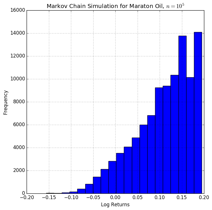

Markov Chain Simulation

Monte Carlo for \(n=10^3 \) iterations

Monte Carlo for \(n=10^4 \) iterations

Monte Carlo for \(n=10^5 \) iterations

Monte Carlo for \(n=10^6 \) iterations

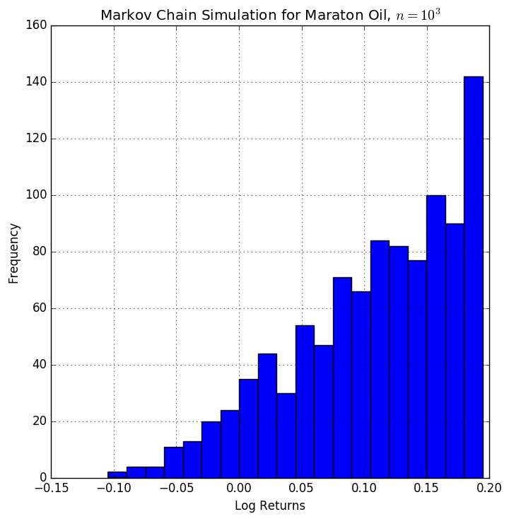
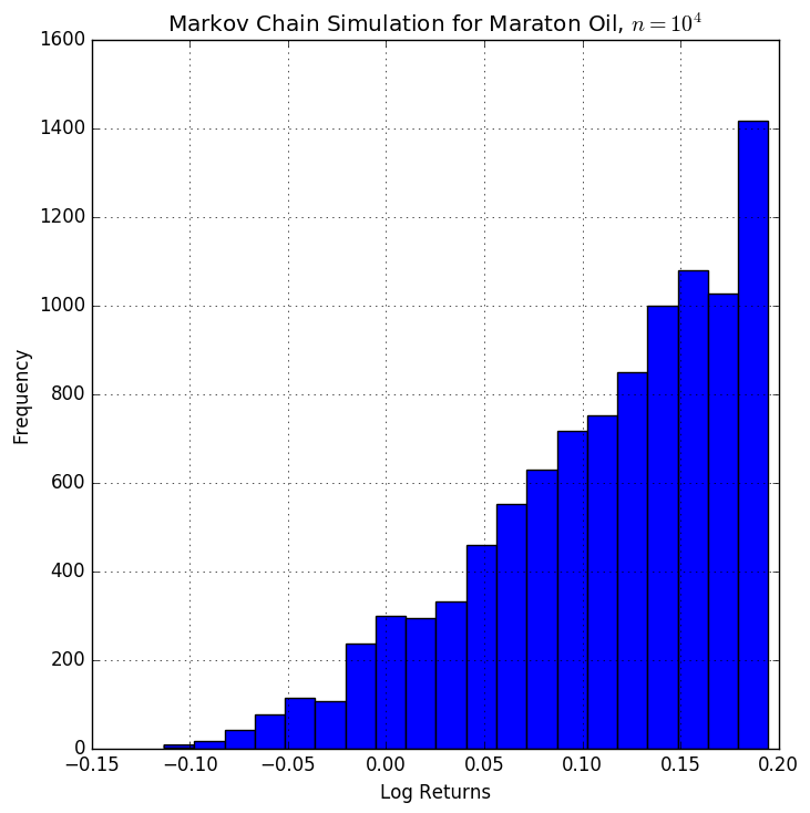
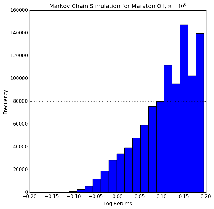
To get bigger images for \(n = \{10^3, 10^4, 10^5, 10^6\}\) iterations, click on the thumbnails above.

Second and N-order Markov Processes

A second order, third order up to \(\text{n}^{th}\) order Markov process behaves the same as described by [smc], except: \[Pr\left(X_t = x_i |X_{t-1},X_{t-2},...,X_{1} \right) = Pr\left( X_t=x_i \right|X_{t-1}=x_{t-1},...,X_{t-n}=x_{t-n})\]

Given observable outcomes, choosing a model is a trade-off between a parsimonious model and a better goodness of fit. Given a likelihood function of the model \(\mathbf{\Lambda}\), once can use a loss function, maximize a probability distribution or use AIC, e.i. \(2k-\ln{\mathbf{\Lambda}}\). Another favourable characteristic of the N-order Markov Processes to be useful in practice is that the transition probability matrix \(\mathbb{A}\) be irreducible.

Any N-order Markovian Process can be represented by a first order Markovian process.

This is rather a trivial proof. Suppose we observe a process that is indeed governed by the function \(f(x,y) \to \mathbb{R}\) where \(x\), \(y\) \(\in\) state spaces \(S,V\) respectively and we want to transform \(f(x,y)\) into \(f(z)\). We can define a state space \(z \in\) \(T = \{(x_i,y_j), \quad x_i \in S \quad y_j \in V \}\) and then rewrite \(f(x,y)\) as \(f(z)\).

Of course the proof goes beyond saying that we can represent any 2-nd order Markov Chains, e.i.: \[Pr\left(X_t |X_{t-1},X_{t-2},...,X_{1} \right) = Pr\left( X_t=x_i |X_{t-1}=x_{t-1},X_{t-2}=x_{t-2} \right)\] as: \[Pr\left(X_t |X_{t-1},X_{t-2},...,X_{1} \right) = Pr\left( X_t=x_i |(X_{t-1},X_{t-2}) \right)\] where \((X_{t-1},X_{t-2})\) is defined as a new state. What the second fundamental theorem of Markov Chains suggests is that even if we have a very complex dynamic process which emits observations \(\epsilon_i\), we can still describe it by a first order Markov chain, given enough states.

Semi Markov Chains and Semi Hidden Markov Models

The SMC and the SHMM are a generalization of the MC and HMM in the sense that they:

1. Allow arbitrarily distributed sojourn times in any state

2. Still have the Markovian hypothesis, but in a more flexible manner.

As defined by Barbu and Limnios (2008)[pp. 2] a process that has these two properties will be called a semi-Markov process.

Continuous State Markov Chains

A continuous state Markov Chain extends the model presented in section [smc] by allowing a probability density distribution on the states. These have been analysed extensively in the paper of Benesch (2001). More formally, a stochastic kernel on \(\mathbb{S}\) is a function \(p:\mathbb{S}\times \mathbb{S}\in \mathbb{R}\) with the property that: \[\begin{aligned} & p(x, y) \geq 0 \quad \forall x,y \in \mathbb{S} \\ & \int_{-\infty}^{+\infty} p(x, y) dy = 1 \quad\forall x \in \mathbb{S}\end{aligned}\]

For example, suppose the random variable \(X_t\) is characterized by the famous normally distributed random walk: \[\label{eq:RWalkNorm} X_{t+1} = X_t + \xi_{t+1} \quad \text{where} \quad \{ \xi_t \} \stackrel {\textrm{ IID }} {\sim} N(0, 1)\]

We could characterize this random distribution through the use of a continuous state Markov Chain, specifically by defining the transition probability \(p(x_t, x_{t+1})\) analogous to \(\mathbb{A}\)³³ to be: \[p(x_t, x_{t+1}) = \frac{1}{\sqrt{2 \pi}} \exp \left\{ - \frac{(x_{t+1} - x_t)^2}{2} \right\}\]

Combining the ideas from the blog of Stachurski and Sargent. (2016) as well as the seminal paper Tauchen (1986) we can connect Stochastic difference equations to the probability kernel. \[\label{eq:genericKernel} X_{t+1} = \mu(X_t) +\sigma(X_t)\xi_{t+1}\] where \(\{ \xi_t \} \stackrel {\textrm{ IID }} {\sim} \phi\) and \(\mu, \sigma\) are functions. This is clearly a Markov process, since the state of the system at \(t+1\) depends only on the current state \(t\). Under this equation, which we will call generic Markov process, we can write the normally distributed random walk stochastic process, as shown in [eq:RWalkNorm] as a special case of equation [eq:genericKernel] when \(\sigma(x_t)=1\) and \(\mu(x_t)=x_t\).

Consider \(X_t\) following an ARCH(1) process: \[\begin{aligned} & y_{t} = a_0 + a_1y_{t-1}+ a_2y_{t-2}+...+a_qy_{t-q-1} + X_t \\ & y_{t+1} = a_0 + a_1y_{t}+ a_2y_{t-1}+...+a_qy_{t-q} + X_{t+1} \\ & X_{t+1} = \alpha X_{t} + \sigma_t \xi_{t+1} \\ & \sigma_t^2 = \beta + \gamma X_t^2, \quad \text{where} \beta, \gamma >0\end{aligned}\]

This is a special case of equation [eq:genericKernel] with \(\sigma(x) = (\beta + \gamma x^2)^{1/2}\) and \(\mu(x) = \alpha x\)

Moreover, it is useful to write equation [eq:genericKernel] in a form of a probability kernel.

Any Markov Process in the form \(X_{t+1} = \mu(X_t) +\sigma(X_t)\xi_{t+1}\) as specified in equation [eq:genericKernel] where \(\xi_{t+1} \sim \phi\) can be written as: \[Pr(x_{t+1}|x_t) = \frac{1}{\sigma(x_t)} \phi \left( \frac{x_{t+1} - \mu(x)}{\sigma(x)} \right)\]

Let \(U\) and \(V\) be two random variables with probability density functions \(f_U(u)\) and \(f_V(v)\) and the cumulative probability distributions \(F_U\) and \(F_V\) respectively and \(V = a+bU\) where \(a,b \in \mathbb{R}\) and \(b>0\). Theorem 8.1.3 from Stachurski and Sargent. (2016) proves that in this case: \(f_V(v)= \frac{1}{b} f_U \left( \frac{v - a}{b} \right)\) and since \(\sigma(x)\) is the square root of \(\sigma^2(x)\) results that \(\sigma(x)>0\) and we can apply Theorem 8.1.3 directly in our case which completes the proof. Proving theorem 8.1.3 from Stachurski and Sargent. (2016) is also straightforward: We know that \(F_V(v) = \mathbb P\{V \leq v \}\), and from the assumption that \(V = a+bU\) we substitute \(V\) and obtain \(F_V(v) = \mathbb P \{ a + b U \leq v \} = \mathbb P \{ U \leq (v - a) / b \}\). We can now write that: \[F_V(v) = F_U ( (v - a)/b )\] and since the probability density function \(f_V(v)\) is the derivative of the cumulative probability distribution \(F_V(v)\) with respect to \(v\), we take the derivative of \(F_V(v)\) and obtain: \[f_V(v) = \frac{1}{b} f_U \left( \frac{v - a}{b} \right)\]

For example, following the Solow-Swan model³⁴ presented in Romer (2006) the capital per capita \(k\) difference equation is: \[\label{eq:SolowK} k_{t+1} = s A_{t+1} f(k_t) + (1 - \delta) k_t\] where

1. \(s\) is the savings ratio

2. \(\delta\) is the normal depreciation rate of the capital

3. \(A_{t+1}\) is the production shock at time \(t+1\) which is latent at time \(t\)

4. and \(f \colon \mathbb R_+ \to \mathbb R_+\) is a production function, usually of the labour augmenting Cobb-Douglas form.

Equation [eq:SolowK] is the driving force of the most popular economic growth model in Economics.³⁵ Since in equation [eq:SolowK] the production shock \(A_{t+1}\) is a random variable, it is also a special case of equation [eq:genericKernel] with \(\mu (x) = (1-\delta)x\) and \(\sigma (x) = sf(x)\). Now we can also write the probability kernel of equation [eq:SolowK] as: \[p(x, y) = \frac{1}{sf(x)} \phi \left( \frac{y - (1 - \delta) x}{s f(x)} \right)\] where \(\phi \sim A_{t+1}\), \(x = k_t\) and \(y=k_{t+1}\).

Having defined the continuous probability transition density, we can generalize the formula for the probability state density at \(t+1\). In the continuous case, if the distribution of \(X_t \sim \psi_t\) then \(\psi_{t+1}\), analogous to the sum as specified in section [smc] for the discrete case: \[\label{eq:CSMC_probVec} \psi_{t+1}(y) = \int p(x,y) \psi_t(x) \, dx, \qquad \forall y \in S\]

Simulating a Continuous State Markov Chain

Once we have established a probability kernel and having the initial probability state distribution \(\psi_0\), we can proceed to estimating the state density distribution \(\psi_1\) at \(t=1\). The straight forward way for simulating the growth of capital as described in equation [eq:SolowK]: \(k_{t+1} = s A_{t+1} f(k_t) + (1 - \delta) k_t\) is to:

1. draw \({k_0}\) from the initial probability density \(\psi_0\)

2. draw \(n\) parameters from the probability density \(\phi\), in the case of the model at equation [eq:SolowK] these are the technology shocks \(A_1 ... A_n\).

3. repeat by computing \(k_{t+1}\) from [eq:SolowK] and store them in an array.

Once we have \(n\) instances of \(k_{t+1}\)s, we can use kernel density estimates functions to make inferences about the probability distribution.³⁶

The paper of Stachurski and Martin (2008), based on the look-ahead estimator, provides an improved Monte Carlo algorithm for computing marginal and stationary densities of stochastic models with the Markov property, establishing global asymptotic normality and fast convergence. The idea is that, by the strong law of large numbers: \[\frac{1}{n} \sum_{i=1}^n p(k_{t-1}^i, y) \to \mathbb E p(k_{t-1}^i, y) = \int p(x, y) \psi_{t-1}(x) \, dx = \psi_t(y)\] where \(p(x,y)\) is the example specific stochastic kernel e.i. \(p(x, y) = \frac{1}{sf(x)} \phi \left( \frac{y - (1 - \delta) x}{s f(x)} \right)\)

Therefore, we can write our continuous state probability density as the average of probabilities: \[\psi_t^n(y) = \frac{1}{n} \sum_{i=1}^n p(k_{t-1}^i, y)\]

Since an efficient implementation of the Monte Carlo simulation for the continuous state Markov process requires a more significant number of steps than in the discrete case, as shown in section [sec:SimMC], and also taking into account that the continuous case is not conceptually different than in the discrete case, providing a step by step implementation as in section is beyond the scope of this thesis. On the other hand, I will present the implementation of Stachurski and Martin (2008) in Julia language in the Annex for convenience purposes.

Given the Solow-Swan model, and using the implementation of the LAE, lae_est as provided in the Annex, we can now ask how fast does the initial density probability function for the continuous state Markov Chain converge to the steady state distribution of capital per capita \(k\). To answer this question we only need to write the function for the probability kernel \(p(x,y)\).

function p(x, y)
              #=
              Stochastic kernel for the growth model with Cobb-Douglas production.
              Both x and y must be strictly positive.
              =#
              d = s * x.^alpha
              pdf_arg = clamp((y .- (1-sigma) .* x) ./ d, eps(), Inf)
              return pdf(phi, pdf_arg) ./ d
          end

The idea is that any initial state density distribution for the \(k_0\) will converge to a steady state density distribution. Suppose the initial density distribution follows: \[f(x; \alpha, \beta) = \frac{1}{B(\alpha, \beta)} x^{\alpha - 1} (1 - x)^{\beta - 1}, \quad x \in [0, 1]\] which is known as the Beta Distribution.

a_sigma = 0.4
          phi = LogNormal(0.0, a_sigma) #Technological Change Distribution
          psi_0 = Beta(1.8, 2.8)
          ygrid = linspace(0.01, 4.0, 200)

fig, ax = subplots()
          #for (x,y) in zip(ygrid, ygrid)
          ax[:plot](ygrid, pdf(psi_0, ygrid), color="0.5")
          t=LaTeXString(" Initial density Distribution: Beta(1.8,2.8) ")
          ax[:set_title](t)
          show()

We can plot the initial distribution of \(\psi_0\)

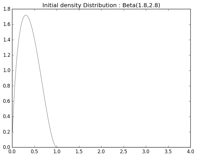
Beta Distribution

and then by iteratively applying the lae function with the density kernel, we can observe the speed of convergence.

s = 0.2 # Savings Rate
          \delta = 0.1 # Capital Depreciation Rate
          a_\sigma = 0.4  # A = exp(B) where B ~ N(0, a_sigma)
          \alpha = 0.4  # We set f(k) = k**alpha
          \psi_0 = Beta(1.8, 2.8)  # Initial Continuous State distribution
          \phi = LogNormal(0.0, a_\sigma)


          n = 10000  # Number of observations at each date t
          T = 30  # Compute density of k_t at 1,...,T+1

          # Generate matrix s.t. t-th column is n observations of k_t
          k = Array(Float64, n, T)
          A = rand!(\phi, Array(Float64, n, T))

          # Draw first column from initial distribution
          k[:, 1] = rand(\psi_0, n)   # divide by 2 to match scale=0.5 in py version
          for t=1:T-1
              k[:, t+1] = s*A[:, t] .* k[:, t].^\alpha + (1-\delta) .* k[:, t]
          end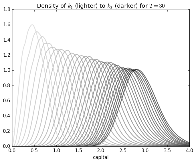

Look Ahead Estimate

Now let us take a more sophisticated probability distribution and observe the convergence. Suppose the initial continuous state distribution follows: \[\begin{split}f(x; \xi, \sigma, \mu) = \begin{cases} \frac{1}{\sigma} \left[ 1+\left(\frac{x-\mu}{\sigma}\right)\xi\right]^{-1/\xi-1} \exp\left\{-\left[ 1+ \left(\frac{x-\mu}{\sigma}\right)\xi\right]^{-1/\xi} \right\} & \text{for } \xi \neq 0 \\ \frac{1}{\sigma} \exp\left\{-\frac{x-\mu}{\sigma}\right\} \exp\left\{-\exp\left[-\frac{x-\mu}{\sigma}\right]\right\} & \text{for } \xi = 0 \end{cases}\end{split}\] for \[\begin{split}x \in \begin{cases} \left[ \mu - \frac{\sigma}{\xi}, + \infty \right) & \text{for } \xi > 0 \\ \left( - \infty, + \infty \right) & \text{for } \xi = 0 \\ \left( - \infty, \mu - \frac{\sigma}{\xi} \right] & \text{for } \xi < 0 \end{cases}\end{split}\] known in the literature as the Generalized extreme value distribution. Unfortunately, this distribution throws an error.

When trying to test the pareto distribution: \[f(x; \alpha, \theta) = \frac{\alpha \theta^\alpha}{x^{\alpha + 1}}, \quad x \ge \theta\] with parameters (3,2), Julia kernel dies.

I have not enough information for the reasons why not all initial distributions converge. I have not tested whether restricting the range will solve this problem or whether there is a bug in the implementations of the distributions.

On the other hand, the most popular distributions do work. For example the Levy distribution. \[\begin{split}f(x; \mu, \sigma) = \sqrt{\frac{\sigma}{2 \pi (x - \mu)^3}} \exp \left( - \frac{\sigma}{2 (x - \mu)} \right), \quad x > \mu\end{split}\]

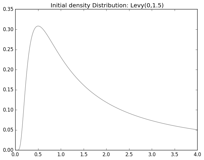
Levy Distribution

after 30 iterations of look ahead estimate with the same parameters as before:

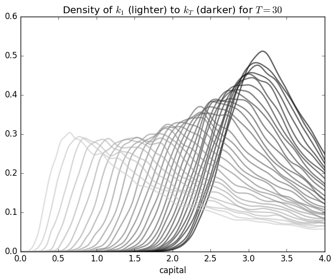
Levy Distribution Convergence

s = 0.2 # Savings Rate
          \delta = 0.1 # Capital Depreciation Rate
          a_\sigma = 0.4  # A = exp(B) where B ~ N(0, a_sigma)
          \alpha = 0.4  # We set f(k) = k**alpha
          \psi_0 = Levy(0,1.5) # Initial Continuous State distribution
          \phi = LogNormal(0.0, a_\sigma)

The conclusion about Continuous State Markov chains is that they are powerful tools to expend point estimates of economic aggregates. As we can see in our example, not only that capital per capita can have a wide range as a function of modest technology shocks, we cannot expect that with time the variance of our distribution will decrease as \(t \to \infty\). In the case of the Levy distribution, we can see that the range the capital per effective capita, as seen in figure [fig:LevyDistConvergence] can increase.

The Hidden Markov Model

A great introduction into the workings of the Hidden Markov processes was presented by Rabiner (1989). In a nutshell, a HMM is defined by a stochastic matrix \(\mathbb{A}\) that changes the the states \(s_i\) of the system according to some probability, where \(s_i \in S\) and \(S\) is the set of all possible States. These states are not observable. Each state can emit some observable outcomes with its own probability distribution which we will summarize in the emission matrix \(\mathbb{B}\). We will take the example given by Fraser (2008, 9).

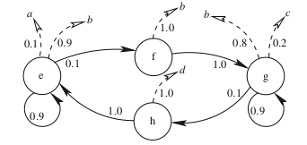
Hidden Markov Model from Fraser (2008, 9)

As we can see in figure [fig:HMM], we have an oriented graph which can easily be transposed to a HMM model.

\[\mathbb{A} = \begin{array}{c} e \\ f \\ g \\ h \end{array} \left( \begin{array}{cccc} 0.9 & 0.1& 0 & 0 \\ 0 & 0 & 1 & 0 \\ 0 & 0 & 0.9& 0.1 \\ 1 & 0 & 0 & 0 \end{array} \right)\]

The emission probabilities for the events \(\Sigma = \{a,b,c,d\}\), as specified in the [smc]: \[\mathbb{B} = \begin{array}{c} e \\ f \\ g \\ h \end{array} \begin{pmatrix} 0.1 & 0.9 & 0 & 0 \\ 0 & 1 & 0 & 0 \\ 0 & 0.8 & 0.2 & 0 \\ 0 & 0& 0& 1 \end{pmatrix}\]

Lastly, to fully define a HMM, we would either need a starting point, or an initial probability distribution among the states usually denoted by \(\pi\).

Having defined a hidden Markov model, we can endeavour to find answers to the following questions:

1. When was the last recession?

2. Are we still in the recession?

3. What is the probability for the economy to follow a particular path of states?

4. What is the unconditional probability of observing certain outcome \(e_i \) or what is the probability of being in a particular state \(s_i\) e \(Pr(S=s_i | e_i)\)?

We conclude that a Hidden Markov Model extends the class of the Markov Chain models, since any order of a Markov model can be represented as an HMM. We will denote a Hidden Markov Model by \(\lambda(\mathbb{A},\mathbb{B},\pi)\).

Simulating a Hidden Markov Model

In this example we will generate a sequence of a balanced and an unbalanced coin that follows an HMM (\(\lambda(\mathbb{A}, \mathbb{B}, \pi)\)) in the Python programming language using the ghmm package. For installing the ghmm library please refer to the Annex and http://ghmm.org. \[\mathbb{A}= \left(\begin{array}{cc} 0.9 & 0.1 \\ 0.2 & 0.8 \\ \end{array}\right)\]

                
                  import ghmm
                  A = [[0.9, 0.1], [0.2, 0.8]]
                  efair = [1.0 / 2] * 2
                  eloaded = [0.15, 0.85]
                  sigma = ghmm.IntegerRange(0,2)
                  B = [efair, eloaded]
                  pi = [0.5]*2
                  m = ghmm.HMMFromMatrices(sigma, ghmm.DiscreteDistribution(sigma), A, B, pi)
                
              

invoking the print method for the HMM model \(m\)

              print m

            DiscreteEmissionHMM(N=2, M=2)
              state 0 (initial=0.50)
                Emissions: 0.50, 0.50
                Transitions: ->0 (0.90), ->1 (0.10)
              state 1 (initial=0.50)
                Emissions: 0.15, 0.85
                Transitions: ->0 (0.20), ->1 (0.80)

generating a sample of 40 observations and printing them.

obs_seq = m.sampleSingle(40)
            obs = map(sigma.external, obs_seq)

            print obs

            [1, 1, 0, 0, 1, 1, 1, 1, 1, 1, 1, 0, 0, 1, 1, 0, 1, 0, 0, 1, 0, 1, 0, 1, 0, 0, 0, 0, 0, 0, 1, 0, 1, 0, 0, 1, 1, 0, 1, 0]

For a dice simulation generated by an HMM, refer to appendix [app:simHMM].

A formal introduction to an HMM

Suppose we have identified a sequence \(\mathcal{O} \in \mathbf{\Omega}\) that we assume is generated by an HMM: \(\lambda(\mathbb{A},\mathbb{B},\pi)\) as defined in chapter [HMM]. Given \(\lambda\), we would like to know: \[Pr(\mathcal{O}|\lambda)=?\]

A direct approach is that given the parameters of the HMM, we can compute the probability of observing a particular observation on a given chain of states: \[\label{eq:basic} Pr\left(o_1,o_2,...,o_{T} |x_1,x_2,...,x_k,...x_T, \lambda \right)= \pi_i b_i(o_1) \prod_{t=2}^{t=T} a_{t-1,t}b_{a_t}(o_t)\]

And then we could sum the probabilities from equation [eq:basic] over all possible states \(X\):

\[\label{eq:directApproach} Pr\left(\mathcal{O} | \lambda \right)= \sum_X \pi_i b_i(o_1) \prod_{t=2}^{t=T} a_{t-1,t}b_{a_t}(o_t) Pr(X|\lambda)\]

Therefore, the direct approach is very difficult to assess. The difficulty of this problem consists in the fact that the total number of possibilities of sequences of states that can generate \(\mathcal{O}\) is exponential in the number of observations \(T\) and would require \(\mathbf{\mathcal{O}}(N^T)\) operations, where \(N\) is the total number of states. At a first glance this might not appear to be a particular big issue in Economics: consider analysing yearly aggregates of a span of 10 years with 2 states \(\Omega = \{Recession, Growth\}\). If, however, we would increase the number of states to 3 and use quarterly data, finding the maximum would require years of computation - clearly not feasible for any practical purpose.³⁷ A better approach to calculate the unconditional probability \(Pr(\mathcal{O}|\lambda)\) is the forward/backward algorithm which is a class of dynamic programming algorithms and takes advantage of the assumptions of the Markovian processes to filter all possible combinations of states \(X\).

Secondly, another question of interest is to find the most likely sequence of states from \(X\) given \(\mathcal{O}\), e.i. the states that generated the highest probability \(Pr(\mathcal{O}| X, \lambda)\).

Finally, the question that sparked my interest in studying Markovian processes is how do we estimate the parameters of an HMM, in particular \(\mathbb{A}\) and \(\mathbb{B}\). Unfortunately, this is still an unsolved problem in Mathematics and requires numerical methods. Once the matrix \(\mathbb{A}\) is determined we can use the dynamic programming and combinatorial methods proposed by Lozovanu and Pickl (2015) for determining the state-time probabilities and the matrix of limiting probabilities. These methods can be directly applied to refine not only the point estimates of long-term economic growth at the country level, as defined by the International Monetary Fond, but also update the concept of long term growth as an integral part of limiting probabilities of a HMM.

To summarize, we could enumerate the key issues we would have to address and solve efficiently for an HMM model to be useful in practice. As expressed by Fraser (2008) and James D. Hamilton and Raj (2002):

1. Evaluation - e.i. find the probability of an observed sequence given an HMM (relatively easy to do in practice)

2. Decoding - find the sequence of Hidden States that most likely generated the observation. That is: find the highest probability of a sequence. (until the Viterbi algorithm it was possible only theoretically)

3. Learning - Generate the best possible HMM for the observed outcome (really difficult - there are no analytic solutions to this problem. Use Baum-Welch algorithm)

The Baum Welch Algorithm

The best way to understand why the Baum-Welch algorithm works is to dissect it into easier algorithms and combine them, until we can answer the questions we posed earlier.

Evaluation

- Use the Forward in combination with Backward algorithm

Decoding

- Viterbi algorithm

Learning

- Use the Bayesian rule along with the Markovian property to update the parameters of the HMM: Baum-Welch algorithm.

The Forward/Backward Algorithm

Given an HMM\((\mathbb{A}, \mathbb{B}, \pi)\), as introduced in section [HMM] which we will denote by \(\lambda(\mathbb{A}, \mathbb{B}, \pi)\), where \(\mathbb{A}\) is the state transition probability e.i. \(a_{ij}=a[i][j]=Pr(x_{t+1}=j|x_t=i)\) and \(\mathbb{B}\) is the emissions probability, e.i. \(b_i(k) = Pr(o_t = k|x_t=i)\),³⁸ and \(\pi\) is the initial probability distribution of states at \(t=1\), e.i. \(\pi_i = Pr(x_1=i)\), where \(i \in \{1..N\}\), the objective of the forward/backward algorithm is to compute the probability of being in a particular state \(x_t\) at time \(t\), given a sequence of observations \(\mathcal{O}\) e.i.: \[Pr(x_k | \mathcal{O})= ? , k \in \{1..T \}\] We can use Bayesian rule³⁹ to write \(Pr(x_k | \mathcal{O} , \mathbf{\lambda})\) as

\[\label{eq:fb1} Pr(x_k | \mathcal{O}, \mathbf{\lambda}) = \frac{Pr(x_k, \mathcal{O} | \mathbf{\lambda})}{Pr(\mathcal{O}|\mathbf{\lambda})} = \frac{Pr(x_k,o_1,o_2,...o_k |\mathbf{\lambda} )*Pr(o_{k+1},...,o_T|x_k,o_1,...o_k,\mathbf{\lambda})}{Pr(\mathcal{O}|\mathbf{\lambda})}\]

Using the Markovian property in the second half of [eq:fb1]⁴⁰ :

\[\label{eq:fb2} Pr(x_k | \mathcal{O}, \mathbf{\lambda}) = \frac{Pr(x_k,o_1,o_2,...o_k |\mathbf{\lambda} ) Pr(o_{k+1},...,o_T|x_k,\mathbf{\lambda})}{Pr(\mathcal{O}|\mathbf{\lambda})}\]

The first part in the numerator of equation [eq:fb2], \(Pr (x_k,o_1,o_2,...o_k |\mathbf{\lambda} )\) is called the forward part and \(Pr(o_{k+1},...,o_T|x_k,\mathbf{\lambda})\) the backward part.

Once we can find an algorithm to compute the forward and the backward part, we can compute \(Pr(x_k | O, \mathbf{\lambda})\) which enables us to answer the following questions:⁴¹

1. The Probability of being in a transition: \(Pr(x_k \not= x_{k-1}|\mathcal{O})\)

2. Helps augment the numerical methods in estimating the parameters of \(\lambda\)

3. Make samples on \(x_k|\mathcal{O}\)

Forward Algorithm

Given an HMM as presented in section [HMM]: \(\lambda(\mathbb{A}, \mathbb{B}, \pi)\), where \(\mathbb{A}\) is the state transition probability e.i. \(a_{ij}=a[i][j]=Pr(x_{t+1}=j|x_t=i)\) and \(\mathbb{B}\) is the emissions probability, e.i. \(b_i(k) = Pr(o_t = k|x_t=i)\),⁴² and \(\pi\) is the initial probability distribution of states at \(t=1\), e.i. \(\pi_i = Pr(x_1=i)\), the objective of the forward algorithm is to compute \[\label{eq:fwa} \alpha_i(k)=\alpha\left( x_k=i \right) = Pr(o_1,o_2,...o_k,x_k | \lambda) \quad\quad o_k \in \mathcal{O}, k=\overline{1,T}\]⁴³

The forward algorithm is also known as the filtering algorithm as it uses the available information up to the point of \(o_k \in \mathcal{O}\). Again, computing \(Pr(o_1,o_2,...o_k,x_k | \lambda)\) directly would require a computation time exponential on \(T\) and would not be feasible for practical purposes. On the other hand, we can use the Law of Total Probability⁴⁴ and the Markov property to express:

If \(k=1\), from the definition of \(\lambda\): \[\alpha(x_k) = \pi_{x_k}\]

else:

\[\begin{aligned} \alpha_i\left( x_k \right) =& \sum_{x_{k-1}} Pr(o_1,o_2,...o_k,x_{k-1},x_k | \lambda) \\ = &\sum_{x_{k-1}} Pr(o_k | o_1,o_2,...o_{k-1},x_{k-1},x_k, \lambda)\times \\&Pr(x_k|o_1,o_2,...o_{k-1},x_{k-1},\lambda) Pr(o_1,o_2,...o_{k-1},x_{k-1}|\lambda) \\ =& \sum_{x_{k-1}} Pr(o_k | x_k, \lambda)Pr(x_k|x_{k-1},\lambda) \alpha\left( x_{k-1} \right) \\ =& \sum_{x_{k-1}} \mathbf{b}_{x_k}(o_k) \mathbf{a}_{(k-1,k)}\alpha\left( x_{k-1} \right) \\ =& \mathbf{b}_{x_k}(o_k) \sum_{x_{k-1}} \mathbf{a}_{(k-1,k)}\alpha\left( x_{k-1} \right) , \quad x_{k-1}=\overline{1,N}, k=\overline{2,T}\end{aligned}\]

Therefore, we can calculate the probability of observing a particular state \(x\) at time \(t\) with a cost of \(\mathcal{O}(N^2T)\) operations using this recursive algorithm which is linear in \(T\), rather than exponential for the naive approach.

Once we have a procedure to efficiently calculate \(\alpha_i(k)\) we can also express the unconditional probability of observing \(\mathcal{O}\) as the sum of all \(\alpha_i(T)\) over all states. \[\label{eq:Pr(O)} Pr(\mathcal{O}|\lambda) = \sum_{i=1}^N \alpha_i(x_T)\]

Backward Algorithm

The backward algorithm is the second part of the forward/backward algorithm in equation [eq:fb2].

As in subsection [sec:fa] we assume that an HMM as presented in section [HMM]: \(\lambda(\mathbb{A}, \mathbb{B}, \pi)\) is given, where \(\mathbb{A}\) is the state transition probability and \(\mathbb{B}\) is the emission probability matrix, e.i. \(b_i(k) = Pr(o_t = k|x_t=i)\) and \(\pi\) is the initial state probability distribution, the objective of the backward algorithm is to compute: \[\label{eq:ba1} \beta_i(k)=\beta(x_k=i) = Pr(o_{k+1},o_{k+2},...,o_{T} | x_k=i, \lambda) \quad i=\overline{1,N}, k=\overline{1,T}\] Again, to get the recursive approach we will make use of the law of total probability to write: \[\begin{aligned} \beta(x_k) =& Pr(o_{k+1},o_{k+2},...,o_{T} | x_k=i, \lambda) \\ =& \sum_{x_{k+1}} Pr(o_{k+1},o_{k+2},...,o_{T},x_{k+1} | x_k=i, \lambda)\end{aligned}\] Now we can divide se sequence of observables and isolate the \(o_{k+1}\) observation as follows: \[\begin{aligned} \beta(x_k) =& \sum_{x_{k+1}} Pr(o_{k+2},...,o_{T}|x_{k+1},x_{k}=i,o_{k+1}, \lambda)\times\\ &Pr(o_{k+1}|x_{k+1},x_{k}=i,\lambda) \times Pr(x_{k+1}|x_{k}=i,\lambda) \end{aligned}\] Now using the Markovian property and the fact that \(Pr(o_{k+1}|x_{k+1},x_{k}=i,\lambda) = Pr(o_{k+1}|x_{k+1},\lambda)\)

\[\begin{aligned} \beta(x_k) &= \sum_{x_{k+1}}\beta(x_{k+1})\mathbf{b}_{k+1}(o_{k+1})\mathbf{a}_{k,k+1}, \quad\quad k=\overline{1,T-1}\end{aligned}\]

The trick in the backward algorithm is that as shown above, \(k\) takes values from \(1\) to \(T-1\). For \(k=T\), we define: \[\beta(x_T)=1\] The intuition for this is clear when applying these algorithms to tagging problems in the Natural Language Programming, since we can define the state of the end of a sentence to be a special symbol “STOP”. And since every sentence ends with this special symbol, the probability of getting \(x_{T+1}=STOP\) equals \(1\).

The Baum-Welch Algorithm

Given an observable sequence \(\mathcal{O} = \{o_1,o_2,...,o_T \}\) and assuming this sequence was generated by an HMM model \(\lambda(\mathbb{A,B},\pi)\) as define in section [HMM], we want to find out the most likely set of parameters of \(\lambda\) that generated the sequence \(\mathcal{O}\). Denoting by \(\theta = \{\mathbb{A,B},\pi\}\) the set of parameters of \(\lambda\), we want to find out \(\theta\) that maximizes the probability:

\[\theta^{\star} = \underset{\theta}{\operatorname{arg\, max}}Pr\left(\mathcal{O} | \lambda(\theta)\right)\]

The Baum-Welch algorithm uses as the basis the EM algorithm, which in turn is very similar to the k-means algorithm.

The first step is to infer the number of states and initial parameters of the \(\lambda(\mathbb{A,B},\pi)\) using heuristic methods.

Secondly, using the forward/backward algorithm as described in section [sec:FBA] from page we find the updated Bayesian probability of observing \(o_t\) at time \(t\) in state \(x_i\) : \[\label{eq:gamma} Pr\left(x_t=i|\mathcal{O},\lambda(\theta)\right) = \frac{\alpha_i(t) \beta_i(t)}{\sum_{j \in S}\alpha_j(t) \beta_j(t) }\] we will denote equation [eq:gamma] by: \[\gamma_i(t) = Pr\left(x_t=i|\mathcal{O},\lambda(\theta)\right)\] please note that in equation [eq:gamma] the denominator \(\sum_{j \in S}\alpha_j(t) \beta_j(t) \) was used rather that a computationally more efficient \(\sum_{i \in S} \alpha_i(x_T) = Pr(\mathcal{O}|\lambda(\theta))\) in order to make \(\gamma_i(t)\) a probability distribution.

Also, using the same backward and forward procedures as described in equation [eq:ba1] and [eq:fwa] we can also compute the probability of switching from state \(x_k=i\) to \(x_{k+1}=j\) given a particular model \(\lambda(\theta)\):

\[\label{eq:xi} Pr(X_t=i,X_{t+1}=j|\mathcal{O},\lambda) = \frac{\alpha_i(t) a_{ij} b_j(o_{t+1}) \beta_j(t)}{Pr(\mathcal{O}|\lambda(\theta))}\]

we will denote equation [eq:xi] by \[\xi_{ij}(t) = Pr(X_t=i,X_{t+1}=j|\mathcal{O},\lambda)\]

Again, we need to make [eq:xi] a probability distribution, and even though it looks computationally attractive to rewrite the denominator as the probability of observing \(\mathcal{O}\) either by the forward or backward algorithm, we cannot write [eq:xi], although wikipedia does⁴⁶, as: \[\xi_{ij}(t) = \frac{\alpha_i(t) a_{ij} b_j(o_{t+1}) \beta_j(t+1)}{\sum_{j\in S} \alpha_j(T)}\] for \(\xi_{ij}(t)\) to be a probability distribution: \[\xi_{ij}(t) = \frac{\alpha_i(t) a_{ij} b_j(o_{t+1}) \beta_j(t+1)} {\sum_{i\in S}\sum_{j\in S} \alpha_i(t) a_{ij} b_j(o_{t+1}) \beta_j(t+1) }\]

Now recall that \(a_{ij}\) is the probability of moving to state \(j\) while already being in state \(i\), e.i. \[a_{ij}= Pr(x_{t+1}=j|x_t=i, \mathcal{O}, \lambda(\theta)\]

We can rewrite the above equation of \(a_{ij}\) by applying the Bayesian rule: \[\label{eq:aij} Pr(x_{t+1}=j|x_t=i, \mathcal{O}, \lambda(\theta) = \frac{Pr(x_{t+1}=j,x_t=i| \mathcal{O}, \lambda(\theta)}{Pr(x_t=i | \mathcal{O}, \lambda(\theta)}\]

Using equations [eq:xi] and [eq:gamma] in equation [eq:aij] we can finally obtain the posterior distribution of \(\bar{a_{ij}}\):

\[\bar{a_{ij}} = \frac{\sum_{t=1}^{T-1}\xi_{ij}(t)}{\sum_{t=1}^{T-1} \gamma_i(t)}\]

equivalently: \[\bar{a_{ij}} = \dfrac{\dfrac{Pr(x_{t+1}=j,x_t=i| \mathcal{O}, \lambda(\theta)}{Pr(x_t=i | \mathcal{O}, \lambda(\theta)}} {\dfrac{\alpha_i(t) \beta_i(t)}{\sum_{j \in S}\alpha_j(t) \beta_j(t) }}\] substituting \[\bar{a_{ij}} = \dfrac{ \dfrac{\alpha_i(t) a_{ij} b_j(o_{t+1}) \beta_j(t+1)} {\sum_{i\in S}\sum_{j\in S} \alpha_i(t) a_{ij} b_j(o_{t+1}) \beta_j(t+1) }} {\dfrac{\alpha_i(t) \beta_i(t)}{\sum_{j \in S}\alpha_j(t) \beta_j(t) }}\] now we have a formula for re-estimating the transition probabilities as a function of the backward and forward probabilities, both of which are linear in \(T\).

To update the initial state probability distribution: \[\bar{\pi_i} = \gamma_1(i) = \frac{\alpha_i(1)\beta_i(1)}{\sum_{i \in S} \alpha_i(1)\beta_i(1) }\]

For the emissions probability we have the expected number of the system being in state \(i\) and observing \(o_k\) : \[\bar{b_i(o_k)} = \frac{\sum_{t \in T} \gamma_t(i) \mathbf{1}_{o_t=o_k}}{\sum_{t \in T} \gamma_t(i)}\]

Therefore, given a model \(\lambda\) , we can compute \(\bar{lambda}(\bar{\mathbb{A}}, \bar{\mathbb{B}}, \bar{\pi})\) and using the results of the theorem provided by Leonard E. Baum and Eagon (1967), specifically:

Let \(P(x) = P (\{x_{ij} \})\) be a polynomial with non-negative coefficients homogeneous of degree \(d\). If \(x_{ij} \geq 0\) and \(\sum_j x_{ij}=1\). Denoting: \[\mathfrak{I}(x)_{ij}= \dfrac{\left( x_{ij} \dfrac{\partial P}{\partial x_{ij}} \middle |_{(x)} \right)} {\left( \sum_j x_{ij} \dfrac{\partial P}{\partial x_{ij}} \right) }\] then \(\mathbb{P}(\mathfrak{I}(x_{ij})) \geq \mathbb{P}(x_{ij}) \)

The proof is provided by Leonard E. Baum and Eagon (1967).

we conclude that \(\bar{\lambda}\) is a better HMM model than \(\lambda\). By •better we mean that \[\mathbb{P}(\mathcal{O}|\bar{\lambda} \geq \mathbb{P}(\mathcal{O}|\lambda)\] Therefore we have obtained an improved version of \(\lambda\). Repeating this process iteratively we will converge to a local maximum. There is no guarantee however that this local maximum will also be a global maximum. Since the optimization surface of a Markov process can be extremely complex, what we can do is randomly assign initial probability distributions \(\mu_i\) for \(i \in \bar{1..n}\) and compare the local optima for each \(i\), hoping we reached the highest value. Most importantly, these new estimated probabilities \(\bar{A}, \bar{B}\) need to make sense, therefore the holistic and heuristic reviews of the most likely models \(\lambda_i\) need to be performed by experts in the field.

The implementation of the Baum Welch algorithm is at the heart of the open source HMM implementation⁴⁷.

To show for convenience purposes how the Baum Welch algorithm works in practice, we will use the data from the example provided by byu.edu⁴⁸, consider the nucleotide sequence \(\{a, c, g, t\}\), assume there is an HMM model \(\lambda(\mathbb{A,B},\pi)\) and the observations \(\mathcal{O}\):

['g', 'c', 'c', 'g', 'g', 'c', 'g', 'c', 'g', 'c', 'g', 'c', 'c', 'g', 'c', 'g', 'c', 'g', 'c', 'g', 'c', 'c', 'g', 'c', 'g', 'c', 'c', 'c','t', 't', 't', 't', 't', 't', 'a', 't', 'a', 'a', 'a', 'a', 't', 't', 't', 'a', 't', 'a', 't', 'a', 'a', 'a', 't', 'a', 't', 't', 't', 't','g', 'c', 'c', 'g', 'g', 'c', 'g', 'c', 'g', 'c', 'g', 'c', 'c', 'g', 'c', 'g', 'c', 'g', 'c', 'g', 'c', 'c', 'g', 'c', 'g', 'c', 'c', 'c','t', 't', 't', 't', 't', 't', 'a', 't', 'a', 'a', 'a', 'a', 't', 't', 't', 'a', 't', 'a', 't', 'a', 'a', 'a', 't', 'a', 't', 't', 't', 't']

generated by two states \(normal, island\). We would like to know what was the sequence of states that generated these observations and would also like to see the most likelihood matrix \(\mathbb{A}\) from the \(\lambda\).

The software implementation is provided in the Annex [app:simHMM].

As we see we have obtained \(\bar{\lambda}\) with updated transition probabilities.

Conclusions

As we have seen in the first part of this thesis Markov Chains have a wide area of applicability in modelling topics in Economics and Finance. Moreover, they provide a fresh paradigm for viewing traditional concepts in Economics such as long term economic growth or stock returns in Finance. The extension of the discrete state Markov chain to continuous states allows us to see the dynamics of the very probability distribution of the variable of interest rather than point estimates. Also, we have seen that the initial distribution assumptions play a crucial role in the variance of subsequent distributions and most importantly, the dispersion not only remains persistent after long periods of time (30 cycles in our case) but it can also increase casting doubt about concepts such as long run equilibrium steady states. On the other hand, Markov Chains are sensitive to how we define and what we incorporate in such abstract concepts as states. Even if we assume that the economy is governed by distinct economic states, it is still a matter of opinion when deciding the number of states. Nevertheless, I avail myself to conclude that the advantages of augmenting a model even with a parsimonious 2 state Markov Model can be expected to yield significant improvements.

A more general model of the Markov Chains that we have discussed in section [HMM], suitable with latent states or imperfect information, is the Hidden Markov Model (also called regime switching model in some sources). It not only allows better fit of traditional econometrics models such as ARMA and ARIMA, it does so using fewer parameters. The drawbacks of the HMM is its complexity and computational requirements in estimating the state transition probabilities. Fortunately, we have concluded that the use of dynamic programming techniques such as the Baum-Welch algorithm, extensively described in [sec:BW] partially solves these problems. The drawback of the Baum-Welch algorithm is that it does not guarantee a global optimum but only a local one and depending on the model, many random iterations of the initial probability distributions are needed to find the parameters of the HMM that generated the observations.

On future work I would like to continue on focusing on Hidden Markov Models and provide solutions to the problem of finding the global optimum. One way is to take advantage of computing parallelism or network distributed systems. This is possible since the bottleneck of estimating the transition probability matrix is in computing power and not in the network of the dimensions of the training set. Using mapreduce functions the central node can easily retain the highest likelihoods and discard others. Furthermore, I would like to further advance the HMM in the continuous state space and allow dimensionality reduction of external variables when defining abstract states of an HMM.

On a more philosophical note, we can conclude that history doesn’t matter for the future if we know the present. Therefore, predicting future returns, especially growth rates, solely on past returns is the wrong path. But do we know the present?

References

A. P. Dempster, D. B. Rubin, N. M. Laird. 1977. “Maximum Likelihood from Incomplete Data via the EM Algorithm.” Journal of the Royal Statistical Society. Series B (Methodological) 39 (1). [Royal Statistical Society, Wiley]: 1–38. http://www.jstor.org/stable/2984875.
Barbu, V.S., and N. Limnios. 2008. Semi-Markov Chains and Hidden Semi-Markov Models Toward Applications: Their Use in Reliability and DNA Analysis. Lecture Notes in Statistics. Springer New York. https://books.google.md/books?id=aNPajwEACAAJ.
Baum, Leonard E, Ted Petrie, George Soules, and Norman Weiss. 1970. “A Maximization Technique Occurring in the Statistical Analysis of Probabilistic Functions of Markov Chains.” The Annals of Mathematical Statistics 41 (1). JSTOR: 164–71.
Baum, Leonard E., and J. A. Eagon. 1967. “An Inequality with Applications to Statistical Estimation for Probabilistic Functions of Markov Processes and to a Model for Ecology.” Bull. Amer. Math. Soc. 73 (3). American Mathematical Society: 360–63. http://projecteuclid.org/euclid.bams/1183528841.
Baum, Leonard E., and Ted Petrie. 1966. “Statistical Inference for Probabilistic Functions of Finite State Markov Chains.” Ann. Math. Statist. 37 (6). The Institute of Mathematical Statistics: 1554–63. doi:10.1214/aoms/1177699147.
Benesch, T. 2001. “The Baum–Welch Algorithm for Parameter Estimation of Gaussian Autoregressive Mixture Models.” Journal of Mathematical Sciences 105 (6). Springer: 2515–8.
Fraser, A.M. 2008. Hidden Markov Models and Dynamical Systems. SIAM E-Books. Society for Industrial; Applied Mathematics (SIAM, 3600 Market Street, Floor 6, Philadelphia, PA 19104). https://books.google.md/books?id=DMEWrB-2gGYC.
Häggström, Olle. 2002. Finite Markov Chains and Algorithmic Applications (London Mathematical Society Student Texts). 1st ed. Cambridge University Press. http://amazon.com/o/ASIN/0521890012/.
Hamilton, James D. 2016. “Macroeconomic Regimes and Regime Shifts.” National Bureau of Economic Research.
Hamilton, James D. 2005. “What’s Real About the Business Cycle?” Working Paper, Working paper series, no. 11161 (February). National Bureau of Economic Research. doi:10.3386/w11161.
Hamilton, James D., and Baldev Raj. 2002. Advances in Markov-Switching Models. Springer Science Business Media. doi:10.1007/978-3-642-51182-0.
Langville, Amy N, and Carl D Meyer. 2011. Google’s PageRank and Beyond: The Science of Search Engine Rankings. Princeton University Press.
Lin, Da, and Mark Stamp. 2011. “Hunting for Undetectable Metamorphic Viruses.” Journal in Computer Virology 7 (3). Springer: 201–14.
Lozovanu, Dmitrii, and Stefan Pickl. 2015. Optimization of Stochastic Discrete Systems and Control on Complex Networks. Springer International Publishing. doi:10.1007/978-3-319-11833-8.
Rabiner, L. R. 1989. “A Tutorial on Hidden Markov Models and Selected Applications in Speech Recognition.” Proceedings of the IEEE 77 (2): 257–86. doi:10.1109/5.18626.
Romer, D. 2006. Advanced Macroeconomics. McGraw-Hill Higher Education. McGraw-Hill. https://books.google.md/books?id=9dW7AAAAIAAJ.
Stachurski, John, and Vance Martin. 2008. “Computing the Distributions of Economic Models via Simulation.” Econometrica 76 (2). The Econometric Society: 443–50. doi:10.1111/j.1468-0262.2008.00839.x.
Stachurski, John, and Thomas J. Sargent. 2016. “Quant Econ Quantative Economics.” http://quant-econ.net/.
Strang, Gilbert. 2011. “18.06SC Linear Algebra.” Massachusetts Institute of Technology: MIT OpenCourseWare. http://ocw.mit.edu/courses/mathematics/18-06sc-linear-algebra-fall-2011/index.htm.
Sundberg, R. 1972. “Maximum Likelihood Theory and Applications for Distributions Generated When Observing a Function of an Exponential Variable.” PhD thesis, PhD Thesis. Institute of Mathematics; Statistics, Stockholm University, Stockholm.
Tauchen, George. 1986. “Finite State Markov-Chain Approximations to Univariate and Vector Autoregressions.” Economics Letters 20 (2). Elsevier BV: 177–81. doi:10.1016/0165-1765(86)90168-0.
see: Langville and Meyer (2011) and Stachurski and Martin (2008),↩
For computer viruses and malware detection using Hidden Markov Models, see (Lin and Stamp 2011)↩
see speech: http://www.math.harvard.edu/ kmatveev/markov.html↩
Analogous to difference equations, we are not interested in the systems dependent on time \(t\) as this will exponentially complicate our estimation technique.↩
In his book, On the Accuracy of Economic Observations (1950), Morgenstern expressed his concerns in the way the data is used from the national income accounts to reach conclusions about the state of the economy and about appropriate policies. Note for Mathematicians: Morgenstern was a friend of John von Neumann.↩
This is probably the reason this adaptation of the EM algorithm is called the Baum-Welch algorithm.↩
We define formally a Markov chain in section [smc]↩
For example, at the Math PISA test \(x_{ij}\) could be whether student \(i\) answered correctly problem \(j\).↩
The National Bureau of Economic Research (NBER) defines recession as “a significant decline in economic activity spread across the economy, lasting more than a few months, normally visible in real GDP, real income, employment, industrial production, and wholesale-retail sales.”, this is a much broader view than simply a decrease in GDP.↩
For example, the Gordon Dividend Discount Model which is augmented with a stream of dividends that are governed by a state transition matrix or a HMM which we will present in section [HMM].↩
which is a fancy way of saying that variables of interest are not always directly observable. Example: Suppose you’re looking for a partner and you want it to be intelligent. The IQ however is not directly observable, and you would have to infer it using his or her behaviour as a function of IQ.↩
Which is a fancy way of saying “observations”. The reason for that can be traced back to the applications of the Markovian processes in speech recognition tasks.↩
We could also think of an zero-order Markov process, the case when the current state is completely independent of the previous state, like throwing a dice. But then we simply get back to a classical probability distribution. If \(\left(\mathbf{\Omega, \Sigma, Pr}\right)\) is a discrete sample space where \(\mathbf{\Omega}\) is the set of all the possible outcomes, \(Pr: \Sigma \mapsto \mathbb{R}\) where \(\sum_{x_{i}\in\mathbf{\Omega}}{Pr(x_{i})} =1\). In this case: \(Pr\left(X_t = x_i |X_{t-1},X_{t-2},...,X_{1} \right) = Pr\left( X_t=x_i \right)\), therefore, it is completely redundant to introduce a zero-order Markov processes.↩
Please note that in a simple Markov Chain, unlike a Hidden Markov Model which we will define later, the states are observable.↩
One of the key insights of this paper is that a linear statistical model with homoskedastic errors cannot capture the nineteenth-century notion of a recurring cyclical pattern in key economic aggregates and that a simple Markov chain has a much better goodness of fit.↩
You can also simulate a Markov Chain given a stochastic matrix at http://setosa.io/ev/markov-chains/↩
period is an abstract term, in the paper of Rabiner (1989) days are assumed, in the example of James D. Hamilton and Raj (2002) months, however for economic aggregates usually quarters are assumed↩
according to a Math professor from MIT (quote needed), this is the second most beautiful series in Math after \(e^x\)↩
other beautiful series derived from the geometric series: http://lycofs01.lycoming.edu/ sprgene/M332/Sums_Series.pdf↩
data from the upstream oil industry as an example↩
In practice it is easier to estimate the profits of a given project in a year given the state of the economy.↩
Octave programming language is very similar to Matlab, except that it is free and open source.↩
The Production Sharing Contracts can be found at http://cabinet.gov.krd/p/p.aspx?l=12&p=1↩
This can be usually found at Article 6 clause 6.9, 6.10, 6.11 and 6.12, for example the Contract signed between Marathon and KRG at http://cabinet.gov.krd/p/p.aspx?l=12&r=296&h=1&s=030000&p=70↩
\(\mathbf{x}\mathbb{A} = \mathbf{x}\) should not be confused with \(\mathbb{A}\mathbf{x} = \mathbf{x}\) since any vector \(\mathbf{x}\) which has \(x_i = x_j\) satisfies this equality.↩
that is \(\mathbf{v}\) is not a zero vector↩
In Octave as well as in other programming languages directly comparing sum(eig(A)) == trace(A) will usually not work due to rounding errors.↩
we will define what irreducible is later.↩
orthogonal is just another way of saying perpendicular or independent vectors↩
the limiting probability matrix is denoted by \(\mathbb{Q}\)↩
Of course we are assuming that the space state transition probability matrix \(\mathbb{A}\) computed by James D. Hamilton (2005) for the United States is valid for Kurdistan Region of Iraq. For these conclusions to have any validity, the study of Hamilton needs to be replicated for KRG and more than 3 states would be desirable to be used.↩
we will present a model when the discount rate is not zero↩
also called stochastic kernel in literature, see for example http://quant-econ.net/jl/stationary_densities.html↩
In a nutshell, the Solow–Swan model assumes a closed market economy. A single good (output) is produced using two factors of production, labour \(L\) and capital \(K\) in an aggregate production function that satisfies the Inada conditions, which imply that the elasticity of substitution must be asymptotically equal to one. https://en.wikipedia.org/wiki/Solow-Swan_model↩
Robert Solow has was awarder the Nobel Prize in Economics.↩
For example the open source library KernelDensity for Julia programming language which is hosted at https://github.com/JuliaStats/KernelDensity.jl↩
For a 2 state economy over a span of 10 years, we would call our function 1024 times, in contrast, a 3 state economy on quarterly data would require 12157665459056928801 (\(1.22*10^{19}\)) calls.↩
usually denoted by \(\varepsilon_i(k)\) in the literature↩
In the appendix I will present the Bayesian rules in probability↩
Since the current outcome depends on the current state and not on past outcomes \(Pr(o_k|x_k,o_{k-1},o_{k-2}...) =Pr(o_k|x_k) \). In practice, it is reasonable to assume that the expected outcome of a function (the growth of Economy) depends on the intrinsic values that define the system, rather than past outcomes.↩
Mathematicalmonk channel present a gentle introduction to HMM and builds intuition what types of questions we can answer https://www.youtube.com/watch?v=7zDARfKVm7s&list=PLD0F06AA0D2E8FFBA↩
I follow the notation of: http://personal.ee.surrey.ac.uk/Personal/P.Jackson/tutorial/hmm_tut2.pdf↩
I used the steps of the algorithm from Wikipedia, https://en.wikipedia.org/wiki/Forward_algorithm except that I corrected for mistakes. For example: Wiki says it uses chain rule, when they meant the law of total probability.↩
Simple as it may sound, according to David Forney↩
https://en.wikipedia.org/wiki/Baum-Welch_algorithm↩
see: http://ghmm.org/↩
link: http://stats.stackexchange.com/questions/70545/looking-for-a-good-and-complete-probability-and-statistics-book↩
link: https://onlinecourses.science.psu.edu/stat414/node/241↩
link: https://www.statlect.com/fundamentals-of-probability/Bayes-rule↩
link: http://stattrek.com/probability/bayes-theorem.aspx↩
link: http://setosa.io/ev/eigenvectors-and-eigenvalues/↩