Applications of Markovian Processes in Economics and Latent Parameters Estimation in Hidden Markov Models

Author: Adrian@Vrabie.net

Adviser: Dr. Habil. Univ Professor Dmitrii Lozovanu

Contens:

1. Introduction
2. Applications of Discrete State Markov Chains in Economics
3. Continuous State Space Markov Chains
4. Part II: Estimating the State Transition Matrix
5. Code Implementation

Introduction

1. Why study Markov Chains?
2. What are Markovian Processes?
3. What types of questions can we answer using Markov Chains?

Applications of Discrete State Markov Chains in Economics

1. First Order Markov Chain
2. Stationary Distribution
3. Simulating a Markov Chain
4. Second and N-order Markov Processes

Continuous State Markov Chains

• Simulating a Continuous State Markov Chain
• Look Ahead Estimate

Part II: Estimating the State Transition Matrix

1. The Hidden Markov Model
2. Simulating a Hidden Markov Model
3. The Forward/Backward Algorithm>
4. The Viterbi Algorithm>
5. The Baum Welch Algorithm

Why study Markov Chains?

Jeffrey Kuan at Harvard University claimed that Markov models might well be the most “real world” useful mathematical concept after that of a derivative.

Why study Markov Chains?

Markovian processes are used in:

• algorithmic music composition
• google search engine
• asset pricing models
• information processing
• machine learning
• computer malware detection
• speech recognition
• nucleotide sequencing
• lung cancer
• and many more

History of Markov Chains

History of Markov Chains from 4m10s

First Order Markov Chain in Music

What is a Markov Chain?

A Markov Chain is:

a dynamic stochastic process with a Markovian Property

What is a Markovian Property?

First order Markov Chain?

First order Markov Chain?

Applications of Markov Chains in Economics

Applications of Markov Chains in Economics

From Hamilton, Economic Transition

With the followint payoffs

The Hamilton Matrix simulation

But We will do this later!

Find Eigenvalues and Eigenvectors of $\mathbb{A}$

This gives us:

We can now calculate the expected payoff conditional on $\mu$

Simulating Marathon Oil Returns

A little bit of Theory

Irreducible Stochastic Matrices

A stochastic matrix, \(\mathbb{A}\) is irreducible if its graph is strongly connected, that is: there \(\exists \; t \geq 0\) : \(Pr(X_{t}=j|X_{0}=i) > 0 \)

In our example, $\mathbb{A}$ is irreducible since we can end up in any state from any state after \(t \geq 1\) steps.

Aperiodic Stochastic Matrices

A stochastic matrix, \(\mathbb{A}\) is aperiodic if the greatest common divisor of the set S(x) defined as \[S(x) = \{t \geq 1 : P^t(x, x) > 0\}\] equals 1.

We can easily check that matrix \(\mathbb{A}\) from our example is aperiodic.

Stationary Distribution

A probability distribution \(\pi\) over \(X\) is stationary over \(\mathbb{A}\) if: \[\pi = \pi \mathbb{A}\]

Fundamental Theorem of Markov Chains

[Fundamental Theorem of Markov Chains][Haggstrom] If a stochastic matrix \(\mathbb{A}\) is irreducible and aperiodic then there is a unique probability distribution \(\pi\) that is stationary on \(\mathbb{A}\).

provided by Häggström (2002).

Therefore, we can write: $$\lim_{t \to \infty} \mu \mathbb{A}^t = \pi$$

Since all but one of the eigenvalues is smaller than unity.

in our example:

The Hidden Markov Model

The Hidden Markov Model

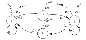
Hidden Markov Model from Fraser (2008, 9)

we have an oriented graph which can easily be transposed to a HMM model.

The Hidden Markov Model

$$\mathbb{A} = \begin{array}{c} e \\ f \\ g \\ h \end{array} \left( \begin{array}{cccc} 0.9 & 0.1& 0 & 0 \\ 0 & 0 & 1 & 0 \\ 0 & 0 & 0.9& 0.1 \\ 1 & 0 & 0 & 0 \end{array} \right)$$

The emission probabilities for the events \(\Sigma = \{a,b,c,d\}\), as specified in the [smc]: \[\mathbb{B} = \begin{array}{c} e \\ f \\ g \\ h \end{array} \begin{pmatrix} 0.1 & 0.9 & 0 & 0 \\ 0 & 1 & 0 & 0 \\ 0 & 0.8 & 0.2 & 0 \\ 0 & 0& 0& 1 \end{pmatrix}\]

An initial probability distribution among the states $\pi$

The Hidden Markov Model

Formally we define an HMM $\lambda(\mathbb{A,B},\pi)$

Parameters, $\mathbb{A,B},\pi$ are often denoted by $\theta$, thus $\lambda(\theta)$

Simulating a Hidden Markov Model

Using external libraries http://ghmm.org.

Emissions: one fair coin and one biased

Outcomes: Head (0) or Tail (1).

[1, 1, 0, 0, 1, 1, 1, 1, 1, 1, 1, 0, 0, 1, 1, 0, 1, 0, 0, 1, 0, 1, 0, 1, 0, 0, 0, 0, 0, 0, 1, 0, 1, 0, 0, 1, 1, 0, 1, 0 ...

The code is provided in the Annex

Forward, Backward and Viterbi Algorithm

Estimating $\lambda(\mathbb{A,B},\pi)$

Before we estimate $\lambda$, it is helpful to answer the following questions:

Evaluation: $Pr(\mathcal{O}|\lambda)=?$

- Use the Forward in combination with Backward algorithm

Decoding: Most likelihood sequence of states $ \texttt{argmax}_{\mathcal{X}} Pr(\mathcal{O}|\mathcal{X},\lambda)=?$

- Viterbi algorithm

Learning: estimate $\lambda$

- Use the Bayesian rule along with the Markovian property to update the parameters of the HMM: Baum-Welch algorithm.

Probability of $\mathcal(O|\lambda)$

Suppose we have identified a sequence \(\mathcal{O} \in \mathbf{\Omega}\) that we assume is generated by an HMM: \(\lambda(\mathbb{A},\mathbb{B},\pi)\). Given \(\lambda\), we would like to know: \[Pr(\mathcal{O}|\lambda)=?\]

Direct approach

Given a model $\lambda$ a sequence of observations $o_1, o_2, ...$ and states $x_1, x_2, ...$

We then sum over all possible states

\[Pr(\mathcal{O}|\lambda)=?\]

The difficulty of this approach is that the total number of possibilities of sequences of states that can generate \(\mathcal{O}\) is exponential in the number of observations \(T\)

\[Pr(\mathcal{O}|\lambda)=?\]

A better approach to calculate the unconditional probability \(Pr(\mathcal{O}|\lambda)\) is the forward/backward algorithm which is a class of dynamic programming algorithms and takes advantage of the assumptions of the Markovian processes to filter all possible combinations of states \(X\).

The Forward/Backward decomposition

the objective of the forward/backward algorithm is to compute the probability of being in a particular state \(x_t\) at time \(t\), given a sequence of observations \(\mathcal{O}\)

The Forward/Backward decomposition

$$Pr(x_k | \mathcal{O}, \mathbf{\lambda}) = \frac{Pr(x_k, \mathcal{O} | \mathbf{\lambda})}{Pr(\mathcal{O}|\mathbf{\lambda})} = $$

$$\frac{Pr(x_k,o_1,o_2,...o_k |\mathbf{\lambda} )*Pr(o_{k+1},...,o_T|x_k,o_1,...o_k,\mathbf{\lambda})}{Pr(\mathcal{O}|\mathbf{\lambda})}$$

using the Markovian property:

$$Pr(x_k | \mathcal{O}, \mathbf{\lambda}) = \frac{Pr(x_k,o_1,o_2,...o_k |\mathbf{\lambda} ) Pr(o_{k+1},...,o_T|x_k,\mathbf{\lambda})}{Pr(\mathcal{O}|\mathbf{\lambda})}$$

The Forward/Backward decomposition

$$Pr(x_k=i | \mathcal{O}, \mathbf{\lambda}) = \frac{\alpha_i(k) \beta_i(k)}{Pr(\mathcal{O}|\mathbf{\lambda})} =$$

$$ \frac{\alpha_i(k) \beta_i(k)}{\sum_{i=1}^N \alpha_i(k=T)} $$

The Forward algorithm

The Backward algorithm

Decoding: The Viterbi Algorithm

Baum Welch algorithm: estimating $\lambda$

Given an observable sequence \(\mathcal{O} = \{o_1,o_2,...,o_T \}\) and assuming this sequence was generated by an HMM model \(\lambda(\mathbb{A,B},\pi)\) we want to find out the most likely set of parameters of \(\lambda\) that generated the sequence \(\mathcal{O}\). we want to find out \(\theta\) that maximizes the probability:

Substituting: $$\bar{a_{ij}} = \dfrac{ \dfrac{\alpha_i(t) a_{ij} b_j(o_{t+1}) \beta_j(t+1)} {\sum_{i\in S}\sum_{j\in S} \alpha_i(t) a_{ij} b_j(o_{t+1}) \beta_j(t+1) }} {\dfrac{\alpha_i(t) \beta_i(t)}{\sum_{j \in S}\alpha_j(t) \beta_j(t) }} $$

example on nucleotides, assuming 2 states:

There is much more:

HTML: Applications of Homogeneous Markovian Processes in Economics and Latent Parameters Estimation for Discrete State Hidden Markov Models

The PDF version (complete)

This presentation: moldovean.github.io

replicate results : github.com/moldovean/usm/tree/master/Thesis

Thank you for your attention!